
CUDA Made Simple: A Short, Practical GPU Programming Guide
A simple, practical guide designed to get you up to speed with CUDA and GPU programming quickly, without unnecessary complexity.

1. Motivation
I recently finished reading Programming Massively Parallel Processors by Hwu, Kirk, and Hajj. It’s a great book, but it’s nearly 600 pages. I couldn’t find a short, comprehensive alternative online, so I wrote this instead.
Why GPUs
CPUs have 8 to 64 cores optimized for sequential, low-latency work. GPUs have thousands of smaller cores built for throughput. An NVIDIA H100 has over 16,000 CUDA cores, all running in parallel. That’s why GPU-accelerated workloads like deep learning training can be orders of magnitude faster.
Why CUDA
CUDA is NVIDIA’s parallel computing platform and the standard way to write GPU code. Most high-performance libraries like cuBLAS and cuDNN are built on top of it. If you want to understand what’s happening inside PyTorch at the metal level, this is where to start.
What this covers
GPU architecture, the memory model, kernels, performance modeling, optimization techniques, algorithms, examples, and more. Enough to build a solid mental model and start writing your own CUDA code.
2. GPU Architecture Fundamentals

Streaming Multiprocessors and cores
A GPU is built around Streaming Multiprocessors (SMs). Each SM has its own CUDA cores, register file, shared memory, and warp scheduler. Work is distributed across SMs, and each SM handles its slice independently.
Thread, block, and grid structure
CUDA organizes work in three levels. A thread is the smallest unit, each running the same kernel on different data. Threads are grouped into blocks, where they can share memory and synchronize. Blocks are grouped into a grid, which is the full set of work for a kernel launch. Blocks and grids can be 1D, 2D, or 3D, making it natural to match your data layout.
Each block always runs on a single SM. The GPU schedules blocks across SMs as resources free up.
Warps and SIMT
Within a block, threads are grouped into units of 32 called warps. The SM schedules warps, not individual threads. All 32 threads in a warp execute the same instruction at the same time, which is the SIMT (Single Instruction, Multiple Threads) model.
If threads in a warp take different code paths, the GPU serializes them. This is called warp divergence and is one of the main performance pitfalls in CUDA.
3. Memory Model
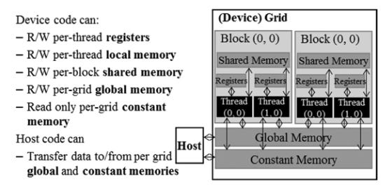
Types of GPU memory
CUDA exposes several memory types, each with different scope, speed, and lifetime:
Global memory: large, slow, accessible by all threads across all SMs. This is the main GPU DRAM.
Shared memory: small, fast, scoped to a block. Threads within the same block can use it to communicate and avoid redundant global memory reads.
Registers: fastest, private to each thread. Used automatically by the compiler for local variables.
Constant memory: read-only, cached, accessible by all threads. Best for values that don’t change during a kernel.
Local memory: private to a thread but physically in global memory. Used when registers spill.
Memory hierarchy and layout
Registers and shared memory live on-chip inside the SM, making them orders of magnitude faster than global memory. Global memory sits off-chip in DRAM and is the main bottleneck in most kernels.
When is the memory allocated?
Registers and shared memory are allocated at kernel launch and freed when the kernel finishes.
Global memory is explicitly allocated and freed by the host using CUDA API calls, and persists across kernel launches.
CUDA memory allocation methods
Data transfer between CPU (host) and GPU (device) goes through PCIe and is slow relative to on-device operations. You want to minimize how often you cross this boundary.
cudaMalloc(&ptr, size); // allocate device (GPU) memory
cudaFree(ptr); // free device memory
cudaMemset(ptr, val, size); // initialize device memory

cudaMemcpy(dst, src, size, cudaMemcpyHostToDevice); // copy memory from host (CPU) to device (GPU)
cudaMemcpy(dst, src, size, cudaMemcpyDeviceToHost); // copy memory from device (GPU) to host (CPU)
Transfers can be made asynchronous using CUDA streams, which allows overlapping compute and data movement. More on that later.
4. Kernels
Host code vs device code
CUDA programs mix two types of code. Host code runs on the CPU and handles things like memory allocation, data transfers, and kernel launches. Device code runs on the GPU and is what actually executes in parallel.
Functions are tagged with qualifiers to tell the compiler where they run:
__global__: runs on the GPU, called from the CPU. This is a kernel.__device__: runs on the GPU, called from the GPU.__host__: runs on the CPU, called from the CPU.
Launching a CUDA kernel
Kernels are launched with a special syntax:
dim3 blockDim(16, 16); // 256 threads per block
dim3 gridDim(W / 16, H / 16); // enough blocks to cover the data
myKernel<<<gridDim, blockDim>>>(args);
gridDim and blockDim can be integers or dim3 structs for 2D/3D layouts. For example:
Thread indexing
Inside a kernel, each thread knows where it is via built-in variables:
int i = blockIdx.x * blockDim.x + threadIdx.x;blockIdx is the block’s position in the grid. threadIdx is the thread’s position within its block. Combined, they give each thread a unique index into your data.
Kernel execution flow
Host calls the kernel with a grid and block configuration.
The GPU runtime distributes blocks across available SMs.
Each SM runs its assigned blocks, one warp at a time.
When all blocks finish, the kernel returns.
Kernel launches are asynchronous by default. The CPU keeps running after the launch. To wait for the GPU to finish, call cudaDeviceSynchronize().
5. The Roofline Model

The Roofline model is a simple way to understand what's limiting your kernel's performance: compute or memory bandwidth.
Arithmetic intensity
Arithmetic intensity is the ratio of floating point operations to bytes of memory traffic (FLOPs / bytes accessed).
A kernel that does a lot of math per byte loaded has high arithmetic intensity. One that loads a lot of data but does little with it has low arithmetic intensity.
Compute-bound vs memory-bound
Every GPU has two hard limits: peak compute throughput (in FLOP/s) and peak memory bandwidth (in GB/s). Dividing them gives you a threshold.
If your kernel’s AI is above that threshold, it’s compute-bound: the bottleneck is the number of operations, and you need to reduce FLOPs or use faster math. If AI is below the threshold, it’s memory-bound: the bottleneck is data movement, and you need to reduce memory traffic or improve access patterns.
Most real-world kernels are memory-bound. Matrix multiplication is one of the few that can be made compute-bound with good tiling.
The roofline gives you a practical ceiling: no matter how well you optimize, you can’t exceed either roof. It tells you which one you’re hitting and where to focus your effort.
6. Key Performance Metrics
Occupancy
Occupancy is the ratio of active warps on an SM to the maximum it can support. Higher occupancy means the SM can better hide memory latency by switching between warps while others wait on data.
Occupancy is limited by register usage, shared memory usage, and block size.
Work per thread
Assigning too little work per thread wastes launch overhead and limits the computation each thread can amortize. Assigning more work per thread (thread coarsening) can improve instruction efficiency, though it reduces parallelism. The right balance depends on your workload.
FLOPs per byte
This is arithmetic intensity in practice. You want each byte you load from global memory to justify itself with as much compute as possible. If you’re loading data and barely using it, memory bandwidth is being wasted.
Control flow divergence
When threads in the same warp take different branches, the GPU serializes the paths and disables threads not on the active path. This reduces the effective parallelism of the warp. The more uniform the control flow across a warp, the better.
7. Optimization Methods
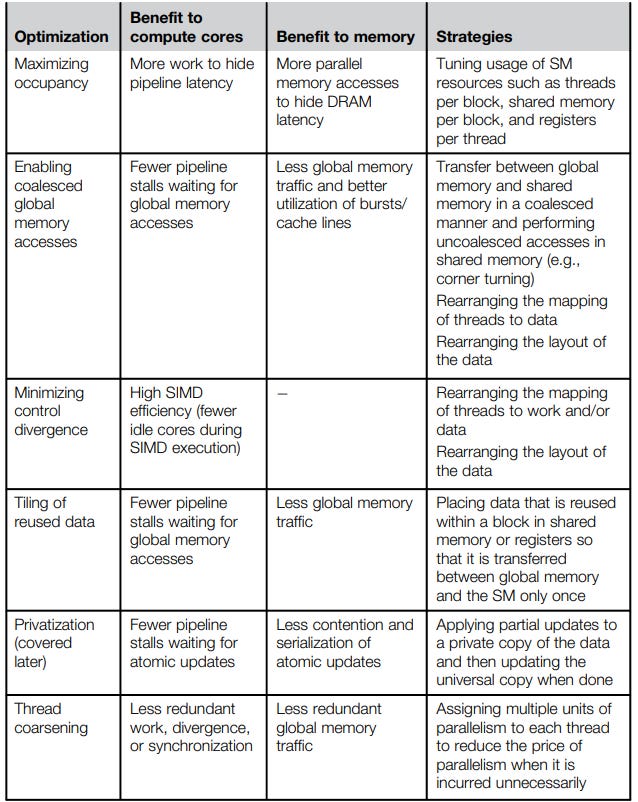
Maximizing occupancy
Reduce register and shared memory usage per thread so more warps can fit on an SM simultaneously.
Coalesced memory access
Global memory is accessed in chunks. When threads in a warp access consecutive memory addresses, those accesses get merged into a single transaction. When they don’t, you pay for multiple transactions. Always try to access memory sequentially across threads in a warp.
float val = data[threadIdx.x]; // coalesced: thread i accesses element i
float val = data[threadIdx.x * stride]; // not coalesced: thread i accesses element i * stride
Minimizing control divergence
Restructure branches so threads in the same warp take the same path. If divergence is unavoidable, try to ensure divergent branches are short.
Thread coarsening
Instead of one thread handling one element, have each thread handle multiple elements. This reduces launch overhead and can improve instruction-level efficiency, at the cost of lower parallelism. Useful when the kernel is already bottlenecked on something other than thread count.
Privatization
Give each thread its own private copy of a shared data structure, have threads accumulate into it locally, then merge results at the end. This avoids contention on shared or global memory. Common pattern in reductions and histograms.
8. Algorithms
The book covers each of these in depth with full CUDA implementations and optimization walkthroughs. We won’t go into details here, but we provide links to efficient CUDA implementations for reference.
Convolution: sliding a filter over input data to produce output values. Foundation of image processing and CNNs.
Stencil: computing each output point from a fixed neighborhood of inputs. Common in finite difference solvers for PDEs and physics simulations.
Histogram: counting occurrences of values across a dataset, with privatization to handle write contention.
Reduction: combining all elements into a single value (sum, max, min) using a tree of parallel operations.
Prefix Sum (Scan): computing running totals across an array. Used as a building block in sorting, compaction, and more.
Merge: combining two sorted sequences into one sorted output in parallel.
Sorting: ordering elements at scale, commonly via parallel radix sort or merge sort.
9. Sparse Data Representations
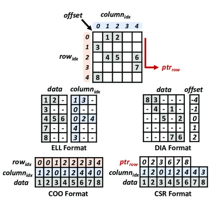
Most real-world matrices in scientific computing and graph processing are sparse, meaning the vast majority of their values are zero. Storing and operating on all those zeros is wasteful, so several compact formats have been developed.
COO (Coordinate Format)
The simplest format. Stores three arrays: row indices, column indices, and values, one entry per nonzero element. Easy to construct but not efficient for computation since there’s no structure to exploit.
CSR (Compressed Sparse Row)
One of the most common format for computation. Instead of storing a row index per element, it stores a row pointer array that marks where each row starts in the values array. This makes row-wise access efficient and maps well to parallel execution where each thread handles a row.
CSC (Compressed Sparse Column)
The column equivalent of CSR. Efficient for column-wise access. Less common but useful for certain operations.
ELL Format
Stores a fixed number of nonzeros per row, padding shorter rows with zeros. This regularity makes it very GPU-friendly since all threads do the same amount of work. The downside is wasted memory when rows have very different nonzero counts.
DIA (Diagonal Format)
Stores the matrix as a set of diagonals, each offset from the main diagonal. Very efficient for matrices that arise from structured grids and finite difference stencils, where nonzeros naturally fall along a small number of diagonals. Wastes space when the nonzero pattern is irregular.
Hybrid Representations
No single format is optimal for all cases. A common approach for graph traversal is to combine ELL and COO: ELL handles rows with a regular nonzero count, and COO handles the outlier rows with many more nonzeros. This avoids the padding waste of pure ELL while keeping most of the access regularity.
10. Problem Decomposition Strategies
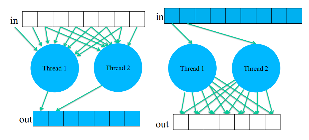
When parallelizing an algorithm, one of the first decisions is how to assign work to threads. There are two fundamental approaches.
Input-centric (Scatter)
Each thread owns a piece of the input and is responsible for writing its contribution to the output. The problem is that multiple threads may need to write to the same output location, requiring atomic operations or other synchronization to avoid race conditions.
Output-centric (Gather)
Each thread owns a piece of the output and reads from wherever in the input it needs to compute its result. This is generally easier to parallelize since each thread writes to exactly one location, with no conflicts. The tradeoff is that the same input element may be read multiple times by different threads.
In practice, output-centric (gather) is the preferred default on GPUs because it avoids write conflicts entirely. However, scatter is sometimes unavoidable.
11. High-Performance Libraries
Writing optimized CUDA kernels from scratch is time-consuming and requires deep hardware knowledge. For common operations, NVIDIA provides highly tuned libraries that are worth using directly.
cuBLAS
NVIDIA’s GPU-accelerated implementation of the BLAS (Basic Linear Algebra Subprograms) standard. Covers dense matrix operations like matrix-matrix multiplication (GEMM), matrix-vector products, and dot products. Under the hood it uses Tensor Cores and other hardware features to get close to peak throughput. PyTorch and TensorFlow both use cuBLAS for their dense linear algebra operations.
cuDNN
NVIDIA’s library for deep learning primitives. Covers convolutions, pooling, normalization, activation functions, etc. Like cuBLAS, it is heavily optimized and is the backbone of most deep learning frameworks. When you run a convolution in PyTorch, cuDNN is doing the actual work.
Both libraries are included in the CUDA Toolkit and expose a C API. They are the right default for production workloads. Writing your own kernels only makes sense when your operation falls outside what these libraries cover, or when you need tighter control over memory layout and fusion.
12. Conclusion
Key takeaways
GPUs are throughput machines. They hide latency through parallelism, not by making individual operations faster.
Most kernels are memory-bound. Where your data lives and how threads access it matters more than arithmetic optimization.
Use the roofline model before optimizing. Know whether you’re compute-bound or memory-bound first.
Warp-level thinking matters. Divergence, coalescing, and occupancy all trace back to how warps behave on the SM.
Use cuBLAS and cuDNN when you can. Only write custom kernels when you have a good reason.
Practical guidance
Get a working kernel first, then profile with Nsight Compute to find the actual bottleneck. Don’t guess.
This guide is meant to be short, intuitive, and complete enough to get you up to speed without reading a textbook. Hopefully it landed that way. For deeper dives on every topic here, including full algorithm implementations and optimization walkthroughs, read Programming Massively Parallel Processors by Hwu, Kirk, and Hajj.